Prasanna

Python Data Persistence – ORM – Filter Criteria

The query object has a filter ( ) method that implements the WHERE clause as used in the raw SQL SELECT statement. The argument to filter can be any Boolean expression. In the following snippet, the filter is ‘price>20000’.

rows=q.filter (Product .price>20000)

This will translate into corresponding SQL statements as under:

Example

SELECT "Products"."ProductID" AS "Products_ ProductID", "Products". 
name AS "Products_name", "Products".price AS "Products_price" 
FROM "Products" 
WHERE "Products".price >?
(20000, )

SQLAlchemy supports the use of wild cards for filter operations on string columns. The LIKE keyword in SQL is implemented by applying a ( ) filter. Products. name. like (‘ %er’) filters rows with product name ending with ‘er’>

rows=q.filter (Product .name. like (1 %er') )

• Python Data Persistence – ORM – Querying
• Python Data Persistence – ORM – Update Data
• Python Data Persistence – Querying Cassandra Table

In effect above statement is equivalent to the following SQL query:

Example

SELECT "Products"."ProductID" AS "Products_ ProductID", 
"Products".name AS "Products_name", "Products".price AS "Products_price" 
FROM "Products" 
WHERE "Products".name LIKE ? 
(' %er' ,)

 

As you will expect, the following output will be displayed:

name: Router price: 2000 
name: Scanner Price: 5000 
name: Printer price: 9000

The filter ( ) can have AND/OR conjunctions implemented by and_ ( ) and or_( ).

Following filter returns products with a price between 10000 and 30000

from sqlalchemy 
import and_ rows=q.filter(and_
(Product.price>10000, Product. price<30000) )

Here is the generated SQL:

Example

SELECT "Products"."ProductID" AS "Products_ ProductID", 
"Products".name AS "Products_name", "Products" .price AS "Products__price" 
FROM "Products" 
WHERE "Products".price > ? AND "Products".price < ? 
(10000, 30000)

The OR operation is performed by the following statement

Example

from sqlalchemy import or_ 
rows=q.filter(or_(Product.price>20000, Product.name. like (' %er' ) ) )

which is equivalent to the following SQL statement:

Example

SELECT "Products"."ProductID" AS "Products_ ProductID", 
"Products".name AS "Products_name", "Products".price AS "Products_price" 
FROM "Products", 
"Customers" WHERE "Products".price <=? 
OR "Customers".name LIKE? 
(5000, '%er')

 

Python Data Persistence – List Comprehension

Python supports many functional programming features. List comprehension is one of them. This technique follows mathematical set builder notation. It is a very concise and efficient way of creating a new list by performing a certain process on each item of the existing list. List comprehension is considerably efficient than processing a list by for loop.
Suppose we want to compute the square of each number in a list and store squares in another list object. We can do it by a for loop as shown below:

Example

#new list with loop
list1= [4,7,2,5,8]
list2= [ ]
for num in listl:
sqr=num*num
list2.append(sqr)
print ('new list:', list2)

The new list will store squares of the existing list.
The list comprehension method achieves the same result more efficiently. List comprehension statement uses the following syntax:

new list = [x for x in sequence]

We use the above format to construct a list of squares by using list comprehension.

• Python Program to Multiply Each Element of a List by a Number | How to Multiply Each Element in a List by a Number in Python?
• Python Program to Print all Perfect Squares from a List using List Comprehension and Math Module
• Python Program to Put Even and Odd elements in a List into Two Different Lists

Example

>>> list1=[ 4 , 7 , 2 , 5 , 8 ]
>>> list2=[num*num for num in list1]
>>> list2
[ 16 , 49 , 4 , 25 , 64 ]
> > >

We can even generate a dictionary or tuple object as a result of list comprehension.

Example

>>> list1= [ 4 , 7 , 2 , 5 , 8 ]
>>> dict1=[{num:num*num} for num in list1]
>>> dict1
[{4 16}, {7: 49}, {2:4}, {5 : 25},{8 : 64 } ]
>>>

List comprehension works with any iterable. Nested loops can also be used in a list comprehension expression. To obtain list of all combinations of characters from two strings:

Example

>>> list1= [x+y for x in 'ABC' for y in ' 123 ' ]
>>> list1
[ 'A1' , 'A2', 'A3', 'B11,' B2 ', 'B3', 'Cl', 'C2', ' C3 ']
>>>

The resulting list stores all combinations of one character from each string.

We can even have if condition in a list comprehension. The following statement will result in a list of all non-vowel alphabets in a string.

Example

>>> consonents=[char for char in "Simple is better
than complex" if char not in [ 'a', 'e' , 'i' , 'o' , 'U' ] ]
>>> consonents
[ 'S' , 'm' , 'p' , '1' , ' ' , 'b' , 't' , 'r' , ' ' , 't' , 'h' , 'n' , ' ' , 'c' , 'm' , 'p' , 'l' , 'x' ]

Conditionals and looping constructs are the two most important tools in a programmer’s armory. Along with them, we also learned about controlling repetition with break and continue statements.
The next chapter introduces the concept of structured programming through the use of functions and modules.

Python Data Persistence – Create Keyspace

As mentioned above. Cassandra Query Language (CQL) is the primary tool for communication with the Cassandra database. Its syntax is strikingly similar to SQL. The first step is to create a keyspace.

A keyspace is a container of column families or tables. CQL provides CREATE KEYSPACE statement to do exactly the same – create a new keyspace. The statement defines its name and replication strategy.

Example

CREATE KEYSPACE name with replication {options}

The replication clause is mandatory and is characterized by class and replication_factor attributes. The ‘class’ decides the replication strategy to be used for the keyspace. Its value is. by default, SimpleStrategy indicating that data will be spread across the entire cluster. Another value of the class is NetworkTopologyStrategy. It is a production-ready strategy with the help of which replication factor can be set independently on each data center.

The replication_factor attribute defines the number of replicas per data center. Set its value to 3, which is considered optimum, so that the data availability is reasonably high.

• Python Data Persistence – Python – Cassandra
• Python Data Persistence – Parameterized Queries
• Python Data Persistence – class Keyword

The following statement creates ‘ My Key Space ’ with ‘ SimpleStrategy’ and a replication factor of 3.

cqlsh> create keyspace my keyspace with
. . . replication={'class': 'SimpleStrategy',
'replication_factor 1 : 3};

Note that, the name of keyspace is case-insensitive unless given in double quotes. CQL provides the use keyword to set a certain keyspace as current. (Similar to MySQL ‘use” statement isn’t it?). To display a list of keyspaces in the current cluster, there is DESCRIBE keyword.

cq1sh> describe keyspaces;
castest            system_auth my keyspace
system_traces
system_schema system           system_distributed
cq1sh> use my keyspace; 
cq1sh:mykeyspace>

Create New Table

As mentioned earlier, one or more column families or tables may be present in a keyspace. The CREATE TABLE command in CQL creates a new table in the current keyspace. Remember the same command was used in SQL?

The general syntax is, as follows:

Example

create table if not exists table_name 
(
col1_definition, 
col2_ definition,
. .
. .
)

Column definition contains its name and data type, optionally setting it as the primary key. The primary key can also be set after the list of columns has been defined. The ‘if not exists” clause is not mandatory but is recommended to avoid error if the table of the given name already exists.
The following statement creates the ‘Products’ table in mykeyspace.

cq1sh:mykeyspace> create table if not exists products
                           . . . (
                           . . . productID int PRIMARY KEY,
                           . . . name text,
                           . . . price int 
                           . . . ) ;

The following definition is also identical:

cq1sh:mykeyspace> create table products
                              . . . (
                              . . . productID int,
                              . . . name text,
                              . . . price int,
                              . . . primary key (productID) 
                              . . . ) ;

Partition Key

Partition key determines on which node will a certain row will be stored. If a table has a single primary key (as in the above definition), it is treated as a partition key as well. The hash value of this partition key is used to determine the node or replica on which a certain row is located. Cassandra stores row having the primary keys in a certain range on one node. For example, rows with a productID value between 1 to 100 are stored on Node A, between 2 to 200 on node B, and so on.

The primary key may comprise more than one column. In that case, the first column name acts as the partition key and subsequent columns are cluster keys. Let us change the definition of the Products table slightly as follows:

cq1sh:mykeyspace> create table products
                                    . . . (
                                    . . . productID int,
                                    . . . manufacturer text,
                                    . . . name text,
                                    . . . price int,
                                    . . . primary key(manufacturer,
productID)
                                   . . . ) ;

In this case, the ‘manufacturer’ column acts as the partition key and ‘productID’ as a cluster key. As a result, all products from the same manufacturer will reside on the same node. Hence a query to search for products from a certain manufacturer will return results faster.

Python Data Persistence – Repetition Control

A looping construct is normally designed to make a certain number of repetitions. For example, the Boolean expression in a while statement decides how many times the block will be repeatedly executed. In the case of for loop, it is decided by the length of iterable.
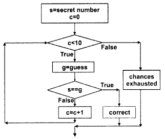
But what if a situation requires early termination of the loop? Consider an example: your program gives the user 10 chances to guess a secret number. Obviously, user input and comparison logic form the body of the loop. However, if the user guesses it right earlier than stipulated chances, naturally the loop should terminate without undergoing all repetitions. Following figure 2.14 explains this scenario:

Python’s break keyword serves exactly this purpose. This keyword appears in a conditional statement inside the loop’s body. If and when the statement evaluates to true, the break statement causes the current loop to be abandoned before the stipulated number of repetitions.
Following Python code implements figure 2.14 flowchart algorithm. To start with a random integer is set as a secret number. (The randint ( ) function is defined in a built-in random module. More about it in the next chapter.) The while loop gives 10 chances for the user to guess it correctly but terminates early if the user gets it right.

• Python Program to Find Next Prime Number
• Python Program to Remove the First Occurrence of Character in a String
• Python Program to Find the Next Armstrong Number

Example

#secret-number.py
import random
secret=random.randint(1,10)
chances=0
while chances<10:
guess = int(input(1 enter your guess..'))
if guess==secret:
print ('you got that right!')
break
print ('try again..')chances=chances+1
if chances==10:
print ('chances exhausted, secret number is : 1,secret)

The output of the above code is shown below. However, your result is likely to be different because a secret number is generated randomly.

Output

E:\python37>python secret-number.py 
enter your guess . . 1 try again . . 
enter your guess . . 2 try again . . 
enter your guess . . 3 try again . . 
enter your guess . . 4 you got that right!

Python also has to continue the keyword which is more or less opposite to break. Instead of breaking out of the current loop, when encountered, continue sends program control back to the beginning of the loop. The remaining statements in the current iteration will not be executed.
A typical scenario of continuing in a loop is like this:
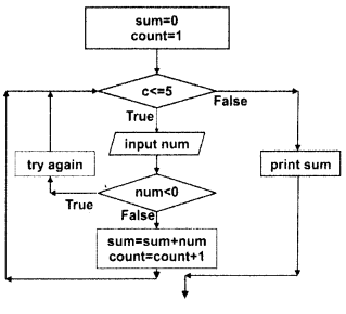
A loop accepts five numbers from the user and displays the sum. However, if a negative number is input, the user is forced to input again. The negative number is kept away from the sum operation. Look at the following flowchart (figure 2.16):

Following Python code implements the above algorithm (figure 2.16).

Example

#continue-example.py
count=1
sum=0
while count<=5:
num=int ( input ( ' enter a number . . ' ) )
if num< 0:
print ('negative number is not accepted. Try again..')
continue
sum=sum+num
count=count+1
print ('sum=',sum)

Output:

E:\python3 7>python continue-example.py 
enter a number . . 2 
enter a number . . 4 
enter a number . . -1 
negative number is not accepted. Try again . .

enter a number . . 6 
enter a number . . -9 
negative number is not accepted. Try again . .

enter a number . . 3 
enter a number . . 1 
sum= 16

E:\python37>

else Statement with Loop

This might be a bit of a surprise to you if you know any C family language (e.g. C, C++, Java, C#, and so on.) The else keyword is normally used to describe the action to be taken when the expression in the if statement is false. While this usage is also defined in Python, else is also used along with looping constructs, both while and for.
When constructing a loop, you can use an optional else block just after the loop’s body. The rest of the statements follow after the else block. The else block comes into play after the loop is over, but before leaving the loop.

Example

#else with loop
while expression==True:
#while block
. .
#end of while block
else:
#else block
. .
#end of else block
#ret of the statements
. .

Following code is typical to use case of else with a loop. The objective is to determine whether the input number is prime or not. The number is successively divided by all numbers between 2 and n. If any number is able to divide it without leaving a remainder, it is a prime. After completion of the loop, else block displays a message of a prime number.

Example

#else-in-loop.py
num=int ( input ( " enter a number . . " ) )
x=2
while x<num:
if num%x==0:
print ("{ } is not prime.".format(num))
break
x=x+1
else:
print ("{ } is prime.".format(num))
print ('end of program')

Note that the else block won’t come into the picture if the loop breaks prematurely as it would happen in case the number is not prime. Here is the output of the above script:

Output:

E : \python37 'python else - in- loop . py 
enter a number . . 31 
31 is prime. end of program 

E:\python37 >python else-in-loop.py 
enter a number . . 24 
24 is not prime. end of program 

E:\python3 7.

It is possible to provide else block for the loop also. You can try writing the above prime number example using for loop.
Hint: You may have to use the range ( ) function in it.

Python Data Persistence – for loop with dictionary

Dictionary object is not iterable as it is an unordered collection of k-v pairs. However, its views returned by methods – items () , keys ( ) , and values ( ) – do return iterables. So, it is possible to use for statement with them. The following code snippet displays each state-capital pair in a given dictionary object.

Example

#for-5.py
dict1={'Maharashtra': 'Bombay', 'Andhra Pradesh': 'Hyderabad', 'UP': 'Lucknow', 'MP': 'Bhopal'}
for pair in dict1.items():
print (pair)

Output:

E:\python37>python for-5.py 
('Maharashtra', 'Bombay') 
('Andhra Pradesh1, 'Hyderabad') 
('UP' , 1 Lucknow') 
('MP' , 1 Bhopal')

 E:\python3 7 >

• Python Data Presistence – Methods of Built-in Data Type Classes
• Data Persistence – Python – PyMongo
• Python: Iterate/Loop over all Nested Dictionary values

As you can see, each pair happens to be a tuple. You can easily unpack it in two different variables as follows:

Example

#for-6.py
dict1={ ' Maharashtra ' : ' Bombay ' , ' Andhra Pradesh ' : ' Hyderabad ' , ' UP ' : ' Lucknow ' , ' MP ' : ' Bhopal ' }
for k ,v in dict1 . items ( ) :
print ( ' capital of { } is { } .'. format ( k , v ) )

Output:

E:\python37>python for-6.py
capital of Maharashtra is Bombay,
capital of Andhra Pradesh is Hyderabad.
capital of UP is Lucknow.
capital of MP is Bhopal.E:\python37>

The keys( ) and values ( ) methods also return iterables. The keys ( ) view returns a collection of keys. Each key is then used to fetch the corresponding value by get ( ) method of the dictionary object.

Example

#for-7.py
dict1={'Maharashtra': 'Bombay', 'Andhra Pradesh': 'Hyderabad', 'UP': 'Lucknow', 'MP': 'Bhopal'}
for k in dict1.keys ( ) :
state=k
capital=dict1.get(k)
print ( 'capital of { } is
{ } .'. format ( state , capital ) )

Python Data Persistence – Program Flow Control

In the previous chapter, although we briefly discussed the scripting mode of the Python interpreter, we mostly worked with Python in interactive mode. It is definitely useful in getting acquainted with the features and syntax of Python especially while learning. It doesn’t prove to be useful though if you want to execute a certain set of instructions repeatedly. In case, if you want to automate a certain process, scripting mode is needed. As we saw in the previous chapter, the script is executed from the command prompt as follows (figure 2.1) :

C:\Users\acer>python hello.py 
enter your name..Akshay 
Hello Akshay how are you?

A program is a set of instructions, which is saved as a script and can be executed together as and when needed. A Python program is simply a text file with .py extension and contains one or more Python statements. Statements are executed in the order in which they are written in script.

Statements in a program follow input-process-output patterns sequentially. However, it is useful only in very simplistic problems, where one or more inputs are collected, processed and, the result of the process is displayed. More realistic and real-world problems require appropriate decisions to be taken depending on varying situations. In other words, we definitely want the program to have a ‘decision’ taking ability.

Many a time an entire process, or a part of it, maybe required to be executed repeatedly until a situation arrives or is encountered. In such a case, the default sequential flow of the program is diverted back to one of earlier statements, thereby constituting a ‘loop’.

• Python Selenium Tutorial | Selenium Python Training for Beginners
• Python Project Ideas & Topics for Beginners to Try in 2021 | Interesting Python Projects List for Beginners, Intermediate, Advanced Level Students
• Python Data Persistence – Installation

The decision statements and looping statements are essential parts of any programming language. In this chapter, you will learn to use Python keywords implementing decision control (if, else, and elif) and repetition control (while and for).

Both these programming constructs, decision and repetition controls are implemented conditionally i.e. based on whether a certain logical expression evaluates to a Boolean value (True or False). Python uses a set of comparison operators to form a logical expression.
The symbols >, <, >=, and <= carry their conventional meaning. The ‘==’ symbol is defined as ‘is equal to’’ operator that returns True if both operands are equal and False otherwise. The ‘!=’ symbol acts as the opposite. It may be called ‘not equal to5 operator

Example

>>> a = 10
>>> b = 5
>>> a > b
True
>>> a < b
False
>>> a>=b*2
True
>>> a*2<=b*4
True
>>> a/2!=b
False
>>>

Repetition

Python’s keywords to construct conditional statements are more or less similar to those found in other languages such as C/C++, Java, and so on. The same is with the repletion control statements. Python has keywords – while and for – using which a loop can be formed in a program. While their usage is similar to that of other languages, there are certain Python-specific changes.
As mentioned at the beginning of this chapter, by default the statements in a program are executed sequentially. However, instead of going to the next instruction, if the program flow redirected to any of the earlier steps, it results in repetitive execution of part of statements in the script.

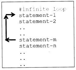
If, as shown in figure 2.5, we somehow manage to make the program go back to statement-1 after statement-m (instead of next in line), the result will be a continuous execution of statements 1 to m which won’t stop on its own and it forms a loop called as an infinite loop. Obviously, this situation is never desired. Instead, we should have a mechanism by which repetition is conditional. The while keyword does exactly the same – it constructs a conditional loop.

Python Data Persistence – Decision Control

Python’s if keyword constructs a conditional statement. It evaluates a boolean expression and executes an indented block of statements following it. The block is initiated by putting the Y symbol after the expression. (Indentation was already explained in the previous chapter.) The following skeleton shows typical usage of if statement and conditional block in a Python script:

Example

#using if statement
if expression==True:
#block of one or more statements
statement 1
statement 2
. . .
. . .
end of if block
#rest of the statements

Let us try to understand this with the help of a simple example. Following script computes tax on employee’s salary @10% if it is greater than or equal to 50,000. No tax is deducted if the salary is less than 50,000.

Example

# tax1 . py
salary= int (input("enter salary . . " ) )
tax=0
if salary>=50000:
#tax @10%
tax=salary*10/100
net_sal=salary-tax
print ("salary={ } tax= { } net payable= { }".
format (salary, tax , net_sal) )

• Python Data Persistence – Querying related tables (ORM)
• Semicolon in Python | How & Why Python Semicolon is Used?
• Python Data Persistence – ORM – Filter Criteria

Save the above script as ‘tax1.py’ and run it from the command prompt as shown below (figure 2.2):

C:\python37>python tax1.py 
enter salary..75000 
Salary=75000 tax=7500.0 net payable=67500.0 

C:\python37>python tax1.py 
enter salary..30000 
Salary=30000 tax=0 net payable=30000 

C:\python3 7 >

Python also provides else keywords. If there is another block of statements to be executed when the expression in if statement happens to be no True (False), it appears as:

Example

#using if statement
if expression==True:
#if block
statement 1
statement 2
. . .
. . .
#end of if block
else:
#else block
statement 1
statement 2
. . .
. . .
#end of else block
#rest of the statements

To show the use of else block, let us modify the previous example of computation of tax, assuming that tax is calculated 5% for salary<50000

Example

#tax2 . py
salary=int (input("enter salary . . " ) )
tax = 0
if salary>=50000:
# tax@10%
tax=salary*10/100
else:
#tax@5%
tax=salary*5/100
net_sal=salary-tax
print ("salary={ } tax={ } net payable = { }".
format (salary, tax, net_sal ) )

Two sample executions of the above script (tax2.py) are as shown below

C:\python37>python tax2.py
enter salary..60000
Salary=60000 tax=6000.0 net payable=54000.0
C:\python37 >python tax2.py
enter salary..20000
Salary=20000 tax=1000.0 net payable;=19000.0

C:\python3 7 >

Python also has elif keyword. Before using it in a Python script, let us modify the above tax calculation program to include few more tax slabs. The tax rate for salary above 50,000 is the same @10%. However, 5% tax is imposed for salary between 25,001 – 50,000. An employee with a salary between 10,001 – 25000 pays 2% tax, and anything below it requires no tax to be deducted. The script looks like as:

Example

#tax3 . py
salary=int ( input ( " enter salary . . " ) )
tax=0
if salary>=50000:
#tax @10%
tax=salary*10/100
else:
if salary>25000 :
#tax @5%
tax=salary*5/100
else:
if salary>10000:
#tax @2%
tax=salary*2/100
else:
#no tax
print ("No tax applicable")
net_sal=salary-tax
print ("Salary={ } tax={ } net payable={ }".
format(salary, tax, net_sal))

Here’s the output showing different tax slabs (figure 2.4)

C:\python37>python tax3.py 
enter salary..60000 
Salary=60000 tax=6000.0 net payable=54000.0 

C:\python37>python tax3.py 
enter salary..40000 
Salary=40000 tax=2000.0 net payable = 38000.0 

C:\python37>python tax3.py 
enter salary..18000 
Salary=18000 tax=360.0 net payable=17640.0 

C:\python37>python tax3.py 
enter salary..5000 
No tax applicable Salary=5000 tax=0 net payable=5000 

E:\python37>

 

While the output is satisfactory as per the expectations, the code (tax3. py) looks a little clumsy because of the increasing indent level of successive if blocks which fall in else part of the previous if statement. This is where the use of elif keyword provides a more elegant way to avoid these indentations and combine empty else with subsequent if block. The general syntax of if- elif- else usage is as shown below:

Example

#using elif statement
if exprl==True:
#first block
. . .
#end of the first block
elif expr2==True:
#second block executes if expr1 is False and expr2 is true.
. . .
#end of the second block
elif exp3==True:
#third block executes if expr2 is false and expr3 is true
. . .
#end of the third block
else:
#else block, executes if all preceding expressions are false
. . .
end of else block
#rest of the statements

In this structure, there is one if block, followed by one or more elif blocks and one else block at the end. Each subsequent elif is evaluated if the previous expression fails. The last else block is run only when all previous expressions turn out to be not true. Importantly all blocks have the same level of indentation. Here, is another version of tax3.py which uses elif blocks.

Example

#tax4.py
salary=int(input("enter salary.."))
tax=0
if salary>=50000:
#tax @10%
tax=salary*10/100
elif salary>25000:
#tax @5%
tax=salary*5/100
elif salary>10000:
#tax @2%
tax=salary*2/100
else :
#no tax
print ("No tax applicable")
net_sal=salary-tax
print ("Salary={ } tax={ } net payable={ }". format(salary, tax, net_sal))

The output of course will be similar to before.

Python Data Persistence – for Keyword

Like many other languages, Python also provides for keywords to construct a loop. However, Python’s for loop is a little different from others. Instead of a count-based looping mechanism, Python’s for loop iterates over each item in a collection object such as list, tuple, and so on.
Python’s sequence-type objects are the collections of items. These objects have an in-built iterator. An iterator is a stream that serves one object at a time until it is exhausted. Such objects are also called iterable. Python’s for loop processes one constituent of an iterable at a time till it is exhausted. The general form of usage of for statement is as follows:

Example

#using for loop
for obj in iterable:
#for block
#processing instructions of each object
. . .
end of block

Unlike the while loop, any other Boolean expression is not required to control the repetition of this block. Let us take a simple example. If you want to calculate the square of each number in a list, use for loop as shown below:

Example

#for-1.py
numbers=[4,7,2,5,8]
for num in numbers:
sqr=num*num
print ( ' sqaure of { } is { } ' . format ( num , sqr ) )

Output:

E:\python3 7 >python for-1.py 
square of 4 is 16 
square of 7 is 49 
square of 2 is 4 
square of 5 is 25 
square of 8 is 64 

E:\python37 >

• Python Program to Find the Minimum Index of a Repeating Element in an Array/List
• Initialize a Python Array – 3 Methods
• Data Persistence – Python – PyMongo

Just like a list, a tuple or string object is also iterable. The following code snippet uses a for loop to traverse the characters in a sentence and count the number of words in it assuming that a single space (‘ ‘)separates them.

Example

#for-2.py
sentence=1 Simple is better than complex and Complex is. better than complicated. '
wordcount=1
for char in sentence:
if char==' ':
wordcount=wordcount+1
print ('the sentence has { } words'.
format(wordcount))

Output

E:\python37>python for-2.py 
the sentence has 11 words 

E:\python37>

Python Data Persistence – Built-in Functions

Python interpreter contains a number of built-in functions. These functions can always be used. You have come across a couple of them in previous sections (type () and id()). In this section, few more built-in functions are being introduced. Some of them will come up for discussion in subsequent chapters. A full list of built-in functions is attached in appendix A.

Number Conversion Functions

A numeric object of one type can be converted to other by using the following built-in functions. These functions have a name that is the same as the built-in data type.

1. int ( ): Function returns an integer from a float or a string of digit characters.

Example

>>> #float to integer
>>> int(10.55)
10
>>> int(0.546)
0
>>> #int from string . .. int('12’)
12

The string of digits returns to an integer according to the decimal number system i.e. base is assumed to be 10. For conversion of string to octal, or hexadecimal integer, the function needs the base – 8 or 16 as the second parameter. Knowing ‘72’ in octal is equivalent to 10 (Ten) and ‘72’ in Hexadecimal is equivalent to 18 (Eighteen). Incidentally, the alphabets ABCDEF are also Hexadecimal digits and hence get converted to their integer equivalents.

• How to Convert a Python String to int
• How to Truncate a float in Python?
• Python Program to Make a Simple Calculator

Example

>>>
int ( '12' ,8)
10
> > > int ('12',16)
18
> > > int ('C',16)
12

2. float ( ): Function returns a floating object from any number or a string containing valid floating-point number representation, either with . decimal point or with scientific notation symbol e or E.

Example

>>> #float from string with decimal notation
. . .
>>> float ( ' 3 .142 ' )
3.142
>>> #float from scientific notation
. . .
>>> float ( ' 1.501E2 ' )
150.1

3. complex( ): Function creates a complex number object out of two parameters given to it. the First parameter is treated as the real part of the complex number and the real part is the second one multiplied by imaginary number j makes up the imaginary part. So, complex(x,y) returns x+yj.

The second argument is optional and is considered 0 by default. Both arguments can be integer, float, or even a complex number.

Example

>>> #complex from integer parameters
. . .
>>> complex(5,6)
(5+6j)
>>> #complex from float parameters
. . .
>>> complex(2.2,-3.5)
(2.2-3.5j)
>>> #complex from complex number parameters
. . .
>>> complex(2+3j,1+2j)
4j

When a second parameter is a complex number, the result is calculated by multiplying it with l+0j and adding the first parameter to it. Hence,

Example

2 + 3j +(1 + 2j)*1 . 0j = 4j

If the first parameter is a string representation of a complex object, there shouldn’t be a second parameter. There shouldn’t be any space within the string.

Example

>>> #complex from string
. . .
>>> complex('1+2j')
(1+2j)
>>> #space not allowed
. . .
>>> complex('1 + 2j')
Traceback (most recent call last):
File "<stdin>", line 1, in <module>
ValueError: complex( ) arg is a malformed string

Conversely real and imaginary components can be separated by a complex number of objects using ‘real’ and ‘imag’ attributes.

Example

>>> c1=complex('1+2j')
>>> #real part
. . .
>>> cl.real
1.0
>>> #imaginary part ... cl.imag
2,0

4. bool ( ): Function evaluates given parameter and returns True or False. It needs one parameter. If it is a non-zero number or an expression that evaluates to a non-zero number, the function returns True, otherwise, it returns False.

Example

>>> #boolean value of integer
. . .
>>> bool(20)
True
>>> bool(-11)
True
>>> bool(0)
Faise
>>> bool(10-5*2)
False
>>> bool(10%2)
False

A non-empty sequence, as well as a dictionary object as a parameter, makes this function True.

Example

>>> #boolean value of sequence
. . .
>>> bool([1,2,3])
True
>>> bool ( [] )
False
>>> bool('') #empty string
False
>>> bool('Hello')
True
>>> bool((1,2,3)) #tuple
True
>>> bool(())
False
>>> bool({1:'one',2:'two'}) #dictionary True
>>> bool({})
False

The bool( ) function also returns True if it receives any logical expression that evaluates to True. Under all other circumstances, bool() returns False.

Example

>>> #boolean value of logical expression
. . .
>>> bool(10>5)
True
>>> bool(3 in [1,2,3,4])
True

Built-in Mathematical Functions

This section introduces some important mathematical functions from the built-in function library.

1. abs ( ): Function returns the absolute value of the parameter, which can be integer, float, or complex number.

Example

>>> #absolute of integer
. . .
>>> abs(-256)
256
>>> #absolute of integer
. . .
>>> abs(1.2E-3)
0.0012
>>> #absolute of complex
. . .
>>> abs(2-3j)
3.605551275463989

2. divmod( ): Function performs division of two parameters and returns division and remainder in the form of a tuple.Absolute value of complex number a+bj is calculated as \(\sqrt{a^{2}+b^{2}}\)

Example

>>> a=divmod(10,3)
> > > a
(3, 1)

3. pow( ): Function performs exponent computation. It takes two numeric parameters. pow(x,y) returns x to the power y (or x raised to y). This is equivalent to exponent operator x**y

Example

>>> pow(10,2)
100
>>> pow(27,1/3)
3.0

4. round ( ): Function returns a number by rounding the parameter to the precision of desired digits before/after the decimal point. the First parameter is the number to be rounded. The second parameter is the digits up to which it is to be rounded. If the digit at the position next to desired precision is greater than 5, then the last digit is increased by 1 and the remaining digits are dropped.

Example

> > > round(123 453467,4)
123.4535
> > > round(123 453467,2)
123.45
>>> round(123 453467,1)
123.5

If the second parameter is 0, then the entire fraction part is considered. If it is greater than 0.5, the return value of the round( ) function is integer part +1, otherwise, only the integer part is returned.

Example

>>> round(123.453467,0)
123.0
>>> round(10/6,0)
2.0

If the second parameter is negative, then the integer part is rounded towards the left of the decimal point.

Example

>>> round(123.453467,-1)
120.0
>>> round(123.453467,-2)
100.0

Sequence Functions

Following functions act on sequence objects (also called tables) such as string, list, and tuple.

1. max ( ): In the case of a list or tuple consisting of numeric items (excluding complex numbers), the largest number is returned. If the list/tuple is made of strings, the one that appears last in alphabetical order is returned. For a string object, the max() function returns a character with the highest ASCII value.

2. min ( ): Function returns the smallest number from list/tuple of numeric items. The string that appears first in alphabetical order is returned by this function if list/tuple is made up of string items. For a single string, the min( ) function returns a character with the lowest ASCII value.

Example

>>>#max/min of numeric items
. . .
>>> tup1=(-50, 3.142,True, 50, pow(8,2) ,1.001e-2)
>>> max(tup1)
64
>>> min(tup1)
-50
>>> #max/min of string items
. . .
>>> list1=['Python', 'Java', 'C++', 'Ruby', 'Kotlin'] >>> max(listl)
'Ruby'
>>> min(list1)
' C++ '
>>> #max/min in a string
. . .
>>> str1='Monty Python and the Holy Grail'
>>> max(str1)
' y'
>>> min(str1)
' '

3. len ( ): In addition to sequence types, this function is also used with dictionary objects. It returns a number of items in sequence/dictionary.

Example

>>> str1='Monty Python and the Holy Grail'
>>> len(str1)
31
>>> list1=['Python', 'Java', 'C++', 'Ruby', 'Kotlin']
>>> len(listl)
5
>>> tup1=(-50, 3.142,True, 50, pow(8,2) ,1.001e-2)
>>> len(tup1)
6
>>> dictl={'Mumbai':'Maharashtra', 'Hyderabad':'Telangana', 'Patna':'Bihar'}
>>> len(dict1)
3

4. list () : Function returns a new list object. If there is no parameter given, an empty list object is created. If a string parameter is used, every character becomes an item in the list object. If a tuple parameter is used, it returns a mutable version of the same items.

Example

>>> list ( )
[ ]
>>> list('Hello Python')
['H' , 'e' , 'l' ,'l' , 'o' , ' ' , 'p' , 'y' , 't' , 'h' , 'o' , 'n']
>>> tup1= ( -50, 3.142, True, 50, pow(8,2),1 001e-2)
>>> list(tup1)
[-50, 3.142, True, 50, 64, 0.01001]

5. tuple ( ): Function returns a new tuple object. If no parameter is given, then an empty tuple object is created. If a string parameter is used, every character becomes an item in the tuple object. If the parameter is a list, it returns an immutable version of the same items.

Example

>>> tuple ( )
( )
>>> tuple('Hello Python')
['H' , 'e' , 'l' ,'l' , 'o' , ' ' , 'p' , 'y' , 't' , 'h' , 'o' , 'n']
>>> list1= (-50, 3.142,True, 50, pow(8,2),1.001e-2)
>>> tuple(list1)
(-50, 3.142, True, 50, 64, 0.01001)

6. str ( ): Function returns a string representation of any Python object. If no parameter is given an empty string is returned.

Example

>>> str ( )
' '
>>> str (1101)
'1101'
>>> str (3.142)
'3.142'
>>> str ([1,2,3])
'[1,2,3]'
>>> str ( (1,2,3))
'(1,2,3)'
>>> str({1: 'one' , 2: 'two' , 3: 'three'})
"{1: ' one ' , 2: 'two' , 3: 'three'}"

Python’s built-in function library has input () and print () functions. The former reads user input and the latter displays output. These functions are meant more for scripting mode rather than interactive mode, although you can them in Python shell as well.10 functions

1. input ( ): When this function is encountered, a Python interpreter waits for input from the input device, the default being the keyboard. The function returns a string object made up of all keys entered by the user until entering the key. You can use a string parameter inside function parentheses to prompt the user about what to input. The return value of the function is usually stored in a string variable for further processing.

Example

>>> name=input( enter your name_')
enter your name: Ramkrishna
>>> name
'Ramkrishna'

2. print ( ): Function displays the value of one or more objects on Python console (if used in interactive mode) or DOS window (if used in scripting mode). In interactive mode, any expression anyway echoes in next line when entered in front of Python prompt >>>.

Example

>>> 2+2
4
>>> print (2+2)
4

This function plays a very important role in displaying output in scripting mode as we shall see soon. There can be multiple comma-separated parameters in the function’s parentheses. Their values are separated by ‘ ‘ although separation character can be changed if you want. For example, if you want ‘,’ between two values, use the sep parameter.

Example

>>> name=' Ram'
>>> age=20
>>> marks= 50
>>> print (name, age, marks)
Ram 20 50
>>> print (name, age, marks, sep=',1)
Ram,20,50

Python scripts become extremely powerful with the use of input() and print() functions. The result of a certain process with different user inputs can be displayed as following: First, using a suitable text editor, type and save the following code as ‘hello.py.

Example

#hello.py
name = input(1 enter your name:')
print ('Hello', name, 'how are you?')

Now, run this script from the command line (figure 1.5):

C : \ Users \ acer>Python hello . py
enter your name:Maya
Hello Maya how are you?

Run it again with different input and get the corresponding output, figure 1.6)

 

C : \ Users \ acer >Python hello . py
enter your name : Mahesh
Hello Mahesh how are you?

 

Remember that the input () function always returns a string object. What if you want numeric input from the user? This is where you have to use different number conversion functions (like int (), float () and so on.) we studied earlier. The following script reads length and breadth from the user and computes the area of a rectangle.

Example

#area.py length=int(input(‘enter length:1)) breadth=int(input(‘enter breadth:’)) area=length*breadth print (‘area=1,area)

Output:

C : \ Users \ acer>Python area . py 
enter length : 20 
enter breadth : 30 area = 600 

C : \ Users \ acer>Python area . py 
enter length : 25 
enter breadth : 35 area : 875

The print ( ) function issues an EOF character (‘\n) at the end. The output of the next print ( ) statement appears below the current line. To make it appear in the same line, specify the ‘end’ parameter to some other characteristics such as ‘ Look at the following modified version of ‘area.py’ script:

Example

#area.py length=int(input(‘enter length:’)) breadth=int (input(‘enter breadth:’)) area=length*breadth print (‘length : ‘ , length, ‘breadth:’ , breadth, end=’ ) print(‘area=’ , area)

Output:

C : \ Users \ acer>Python area . py
enter length : 20
enter breadth : 30
length : 20 breadth : 30 area = 600

Python Data Persistence – Python – PyMongo

is NOSQL?

In today’s era of real-time web applications, NoSQL databases are becoming increasingly popular. The term NoSQL originally referred to “non SQL” or “non-relational”, but its supporters prefer to call it “Not only SQL” to indicate that SQL-like query language may be supported alongside.

NoSQL is touted as open-source, distributed, and horizontally scalable schema-free database architecture. NoSQL databases are more scalable and provide superior performance as compared to RDBMS. This primarily because it requires that schemas (table structure, relationships, etc.) be defined before you can add data. Some of the popular NoSQL databases extensively in use today include MongoDB, CouchDB, Cassandra, HBase, etc.

Several NoSQL products are available in the market. They are classified into four categories based on the data model used by them.

Key-Value store: Uses a hash table (also called a dictionary). Each item in the database is stored as a unique attribute name (or ‘key’), associated with its value. The key-value model is the simplest type of NoSQL database. Examples of key-value databases are Amazon SimpleDB, Oracle BDB, Riak, and Berkeley DB.

Column Oriented: This type of databases store and process very large amount of data distributed over multiple machines. Keys point to multiple columns. The columns are arranged by column family. Examples of column-oriented databases are Cassandra and HBase.

Document oriented: Database of this category is an advanced key-value store database. The semi-structured documents are stored in formats like JSON. Documents can contain many different key-value pairs, or key- array pairs, or even nested documents.

Graph Based: Databases of this type are used to store information about networks of data, such as social connections. A flexible graph model can scale across multiple machines. Graph stores include Neo4J and Giraph.
In this chapter, we shall get acquainted with a hugely popular document-oriented database, MongoDB, and how it can be interfaced with Python through the PyMongo module.

• Python Data Persistence – PyMongo – Relationships
• Python Data Persistence – A Quick Guide
• Python Data Persistence – Python – Cassandra

MongoDB

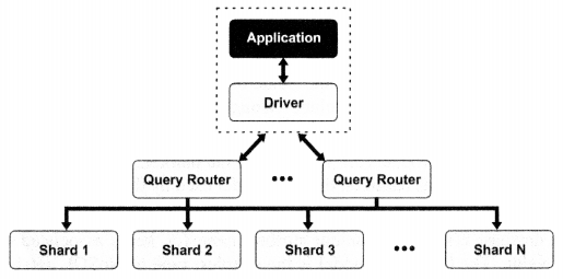
NoSQL databases typically have a huge amount of data. Hence, more often than not, the power of a single CPU is not enough when it comes to fetching data corresponding to a query. MongoDB uses a sharding technique that splits data sets across multiple instances. A large collection of data is split across multiple physical servers called ‘shards’, even though they behave as one collection. Query request from the application is routed to the appropriate shard and the result is served. Thus, MongoDB achieves horizontal scalability, (figure 11.1)

The Document is the heart of a MongoDB database. It is a collection of key-value pairs – similar to Python’s dictionary object. We can also think of it being similar to a single row in a table of SQL-based relational databases.

Collection in MongoDB is analogous to a table in the relational database. However, it doesn’t have a predefined schema. The Collection has a dynamic schema in the sense each document may of a variable number of k-v pairs not necessarily with the same keys in each document.

Each document is characterized by a special key called “_id” having a unique value, again similar to a primary key in the entity table of a relational database.

MongoDB server has a command-line interface from inside which different database operations can be performed.

MongoDB – Create Database

To display the current database in use, there’s a DB command. The default database in-use tests.

> db 
Test

With the ‘use’ command any other database is set as current. If the named database doesn’t exist, a new one is created.

> use mydb 
switched to db mydb

However, until you store data(such as collection or document) in it, is the database is not created. The following command inserts a document in the ‘products’ collection under the current database.

MongoDB – Insert Document

Appropriately, insertone ( ) method is available to a collection object in a database. A document is provided to it as a parameter.

> db.products.insertone({"ProductID":1, 
"Name":"Laptop", "Price":25000}) 
WriteResult({ "nlnserted" : 1 })

Result of above (for that matter any insert/update/delete operation) command returns WriteResult object. The insert () method inserts multiple documents if the argument is an array of documents. In that case, the result is BulkWriteResult object.

> var pricelist=[{'productID' :1, 'Name': 'Laptop' , 'price':25000}, 
. . . { 'productID' : 2, 'Name":'TV' , 'price':2000}, 
. . . { 'productID' : 3, 'Name":'Router' , 'price':2000}, 
. . . { 'productID' : 4, 'Name":'Scanner' , 'price':5000}, 
. . . { 'productID' : 5, 'Name":'Printer' , 'price':9000}, 
> db.products.insert(pricelist); 
BulkWriteResult ({
 "writeErrors" : [ ] , 
 "writeConcernErrors" : [ ] , 
 "nInserted" : 5 , 
 "nUpserted" : 0 , 
 "nMatched" : 0 , 
 "nModified" : 0 , 
 "nRemoved" : 0 , 
 "upserted" : [ ] 
 })

The insert () function inserts a single document or array whereas a single document is inserted with inserOne ( ) method and array whereas the insert_many () method is used with an array.

MongoDB – Delete Document

The remove () method deletes one or more documents from the collection based on the provided criteria. The following statement will result in the removal of a document pertaining to price>40000 (in our data it happens to be with name=’TV’).

> db.products.remove({"price":{$gt:40000}}) 
WriteResult({ "nRemoved" : 1 })

Run the find ( ) method in the shell to verify the removal.

Now that, we have attained some level of familiarity with MongoDB with the help of shell commands. Let us concentrate on our main objective – use MongoDB in Python.

PyMongo – Update Document

PyMongo offers two collection methods for the modification of data in one or more documents. They are update_one () and update_many () . Both require filter criteria and a new value of one or more keys. The update_one () updates only the first document that satisfies filter criteria. On the other hand, update__many () performs updates on all documents that satisfy the filter criteria.

collection.update_one (filter, newval)

Following Python script accepts the name of the product from the user and displays the current price. It is updated to the new price input by the user.

Example

> var pricelist=[{'productID' :1, 'Name': 'Laptop' , 'price':25000}, 
. . . { 'productID' : 2, 'Name":'TV' , 'price':2000}, 
. . . { 'productID' : 3, 'Name":'Router' , 'price':2000}, 
. . . { 'productID' : 4, 'Name":'Scanner' , 'price':5000}, 
. . . { 'productID' : 5, 'Name":'Printer' , 'price':9000}, 
> db.products.insert(pricelist); 
BulkWriteResult ({
 "writeErrors" : [ ] , 
 "writeConcernErrors" : [ ] , 
 "nInserted" : 5 , 
 "nUpserted" : 0 , 
 "nMatched" : 0 , 
 "nModified" : 0 , 
 "nRemoved" : 0 , 
 "upserted" : [ ] 
 })

Python Data Persistence – pyMongo – Querying Collection

PyMongo module defines find( ) method to be used with a collection object. It returns a cursor object which provides a list of all documents in the collection.

>>> products=db['products']
>>> docs=products .find ()
>>> list(docs)
[{'_id' : Objectld('5c8dec275405cl2e3402423c'),
'ProductID': 1, 'Name': 'Laptop', 'price': 25000},
{'_id': ObjectId('5c8dec275405cl2e3402423d'),
'ProductID': 2, 'Name': 'TV', 'price': 50000},
{'_id': Objectld('5c8dec275405cl2e3402423e'),
'ProductID': 3, 'Name': 'Router', 'price': 2000},
{'_id': Objectld('5c8dec275405cl2e3402423f'),
'ProductID': 4, 'Name': 'Scanner', 'price': 5000},
{'_id': Objectld('5c8dec275405cl2e34024240'),
'ProductID': 5, 'Name': 'Printer', 'price': 9000}]

This cursor object is an iterator that serves one document for every call of the next () method. Each document is a dictionary object of k-v pairs. The following code displays the name and GSTIN of all customers.

Example

#mongofind. py 
from pymongo import MongoClient 
client=MongoClient( ) 
db=client.newdb 
cust=db['customers'] 
docs=cust. find ( ) 
while True:               
 try:                          
         doc=docs.next()                          
         print (doc['Name'], doc['GSTIN'])              
         except Stoplteration:                           
         break 
 client.close ( )

Run the above script from the command prompt.

E : \python3 7 >python mongofind. py
Ravikumar 27AAJPL7103N1ZF
Patel 24ASDFG1234N1ZN
Nitin 27AABBC7895N1ZT
Nair 32MMAF8963N1ZK
Shah 24BADEF2002N1ZB
Khurana 07KABCS1002N1ZV
Irfan 05IIAAV5103N1ZA
Kiran 12PPSDF22431ZC
Divya 15ABCDE1101N1ZA
John 29AAEEC4258E1ZK

You can, of course, employ a regular ‘for’ loop to traverse the cursor object to obtain one document at a time.

Example

for doc in docs: 
      print (doc['Name'] , doc[1GSTIN'])

The logical operators of MongoDB (described earlier in this chapter) are used to apply filter criteria for the find ( ) method. As an example, products with price>10000 are fetched with the following statement:

Example

>>> products=db['products'] 
>>> docs=products .find 
({'price :{ 1$gt ' :10000} } ) 
>>> for 
doc in docs: print (doc.get('Name'), 
doc.get('price')) Laptop 25000 TV 50000