Prasanna

Python Data Persistence – PyMongo Module

PyMongo module is an official Python driver for MongoDB database developed by Mongo Inc. It can be used on Windows, Linux, as well as MacOS. As always, you need to install this module using the pip3 utility.

pip3 install pymongo

Before attempting to perform any operation on a database, ensure that you have started the server using ‘mongod’ command and the server is listening at port number 22017.

To let your Python interpreter interact with the server, establish a connection with the object of MongoClient class.

• Data Persistence – Python – PyMongo
• Python Data Persistence – MongoDB – Update Document
• Python Data Persistence – SQLAlchemy Core

Example

>>> from pymongo import MongoClient 
>>> client=MongoClient( )

The following syntax is also valid for setting up connection with server.

>>> client = MongoClient('localhost', 27017)
#or
client = MongoClient('mongodb://localhost:27017')

In order to display currently available databases use list_database_ namesO method of MongoClient class.

Example

>>> client.list_database_names( )
[' admin' , ' config' , 1 local' , ' mydb' ]

Python Data Persistence – User-defined Types

While executing the queries, Python data types are implicitly parsed to corresponding CQL types as per the following table:(figure 12.1)

Python Type	CQL Type
None	NULL
Bool	Boolean
Float	Float, double
Int, long	Int, bigint , variant , smallest, tinyint , counter
Decimal, decimal	Decimal
Str , Unicode	Ascii, varchar , test
Buffer, byte array	Blob
Date	Date
Datetime	Timestamp
Time	Time
List , tuple Generator	List
Set , frozenest	Set
Dict , OrderedDist	Map
Uuid.UUID	Timeuuid.uuid

• Data Persistence – Python – PyMongo
• Python Data Persistence – RDBMS Concepts
• Program to Handle Precision Values in Python

In addition to the above built-in CQL data types, the Cassandra table may have a column of a user-defined type to which an object of Python class can be mapped.

Cassandra provides a CREATE TYPE statement to define a new user-defined type which is used as a type for a column in a table defined with the CREATE TABLE statement.

In the script given below (Cassandra-udt.py), we define a Cassandra user-defined type named ‘contacts’ and use it as the data type of the ‘contact’ column in the ‘users’ table. The register__user_type ( ) method of cluster object helps us to map Python class ‘Contactlnfo’ to the user-defined type.

Example

#cassandra-udt.py 
from cassandra.cluster import Cluster 
cluster = Cluster(protocol_version=3) 
session = cluster.connect( ) 
session.set_keyspace(1mykeyspace1) 
session.execute("CREATE TYPE contact (email text, phone text)") 
session.execute("CREATE TABLE users (userid int PRIMARY KEY, name text, contact frozen<contact>)") 
class Contactlnfo:          
      def__init__(self, email, phone):                       
           self.email = email                       
            self.phone = phone 
cluster.register_user_type('mykeyspace', 'contact', Contactlnfo) 
# insert a row using an instance of Contctlnfo session.execute("INSERT INTO users (userid, name, contact) 
VALUES (%s, %s, %s)",                           
   (1, .'Admin', Contactlnfo
("admin@ testserver.com", '9988776655')))

The following display of the CQL shell confirms the insertion operation of the above script.

cq1sh:mykeyspace> select * from users; 
    userid          |                            contact                                            |  name
------------+------------------------------------------------------------+-----------
        1        | {email: 'admin@testserver.com', phone: '9988776655'}  |   Admin 
(1 rows)

In this chapter, we learned about the basic features of the Cassandra database, and importantly how to perform read/write operations on it with Python.

Final thoughts

This is also the last chapter of this book. Starting with the basics of Python, we learned how to work with different data storage formats. This work is neither a Python handbook nor a SQL/NoSQL database guide. Instead, it is intended to be a simple and practical explanation of Python interfaces with different data persistence avenues available today.

This book concentrates primarily on basic CRUD operations on SQL and NoSQL databases and other data file formats. However, these techniques are merely complementary to the real data crunching a data scientist needs to perform. The next logical thing for a curious reader would be to acquire data manipulation and visualization skills for which Python has very rich and powerful libraries.
1 hope you enjoyed this book as much as 1 did bring to you. Feedback, suggestions, and corrections if any are most welcome so that subsequent editions can be improved.
Thanks.

Python Data Persistence – MongoDB – Querying Collection

Retrieving data from the database is always an important operation. MongoDB’s collection has found ( ) method with which documents are fetched. Without any argument, the find ( ) method returns a result set of all documents in a collection. In effect, it is equivalent to ‘SELECT * FROM <table>‘ in SQL.

> db . products . find () 
{ "_id" : Objectld("5c8d420c7bebaca49b767db3"), 
"ProductID" : 1, "Name" : "Laptop", "price" : 25000 
} 
{ "_id" : Objectld("5c8d420c7bebaca49b767db4"), 
"ProductID" : 2, "Name" : "TV", "price" : 40000 } 
{ "_id" : Objectld("5c8d420c7bebaca49b767db5"), 
"ProductID" : 3, "Name" : "Router", "price" : 2000 } 
{ "__id" : Objectld("5c8d420c7bebaca49b767db6"), 
"ProductID" : 4, "Name" : "Scanner", "price" : 5000 } 
{ "_id" : Objectld("5c8d420c7bebaca49b767db7"), 
"ProductID" : 5, "Name" : "Printer", "price" : 9000 
}

Note that, ‘_id’ key is automatically added to each document. The value of each _id is of ObjectId type and is unique for each document.
Invariably, you would want to apply to the result set returned by find ( ). It is done by putting the key-value pair in its parenthesis. In its generalized form, the conditional query is written as follows:

Example

db. collection .find ({ "key" : "value"})

The following statement retrieves a document whose ‘Name’ key has ‘TV’ value.

• Data Persistence – Python – PyMongo
• Python Data Persistence – MongoDB – Update Document
• Python Data Persistence – ORM – Querying

Example

> db .products .find ({"Name": "TV"}) 
{ "_id" : Objectld("5c8d420c7bebaca4 9b76 7db4"), 
"ProductID" : 2, "Name" : "TV", "price" : 40000 }

MongoDB doesn’t use traditional logical operator symbols. Instead, it has its own operators, as listed below:

The operators are used in the find ( ) method to apply the filter. The following statement returns products with a price> 10000.

> db.products .find ({"price" : {$gt: 10000 }}) 
{ 
"_id" : Objectld("5c8d420c7bebaca49b767db3"), 
"ProductID" : 1, "Name" : "Laptop", "price" : 25000 
} 
{ "_id" : Objectld("5c8d420c7bebaca49b767db4"), 
"ProductID" : 2, "Name" : "TV", "price" : 40000
}

The Sand, as well as Sor operators, are available for compound logical expressions. Their usage is, as follows:

Example

db. collection.find ($and: [ {"keyl" :"value 1"},
{"key2":"value2"} ] )

Use the following command to fetch products with prices between 1000 and 10000.

> db . products . find ( { $and: [ { "price" : { $gt: 1000 } } , {"price":{$lt:10000}} ] }) 
{ "_id" : Objectld("5c8d420c7bebaca49b767db5 " ) , 
"ProductID" : 3, "Name" : "Router", "price" : 2000 
} 
{ "_id" : Objectld("5c8d420c7bebaca49b767db6"), 
"ProductID" : 4, "Name" : "Scanner", "price" : 5000 
} 
{ "_id" : Obj ectld("5c8d42 0c7bebaca4 9b767db7") ,
 "ProductID" : 5, "Name" : "Printer", "price" : 9000
}

 

Python Data Persistence – Charts

One of the most attractive features of the MS Excel application is to dynamically generate various types of charts based upon data in worksheets. The openpyxl package has a chart module that offers the required functionality. In this section, we shall see how we can render charts programmatically.

The chart module defines classes for all types of charts such as BarChart and LineChart. The chart requires data range and category range to be defined. These ranges are defines with the Reference () function. It stipulates row and column numbers of top-left and bottom-right cells of the desired range.

In the above worksheet, B2:D7 is the data range including the column labels, and A1: A7 range is the categories range.

• Data Persistence – Python and Excel
• Python Data Persistence – Read Data from Worksheet
• Python Pandas DataFrame plot.barh() Function

Example

from openpyxl import load_workbook 
wb = load_workbook(1 example.xlsx') 
ws = wb.active 
from openpyxl.chart import BarChart, Reference 
values = Ref erence (ws, min_col=2, min__row=2, max_ col=4, max_row=7) 
ctg=Reference(ws, min_col=l,min_row=3, max_col=l, max_row=7)

The chart object is configured by add_data() and set_ categories ( ) methods. The add_data() method takes the data range as the first parameter. If the titles_f rom_data parameter is set to True, the first row in the data range is used for the series legend title. The title of the chart, X-axis and Y-axis are also set by respective properties.

Example

c1 = BarChart( )
c1.add_data(values, titles_from_data=True
c1 . title = "Bar Chart"
c1.x_axis.title = 'Months1
c1. y__axis . title = 'Sales'
ws . add__chart (cl, "A10")
c1.set_categories(ctg)
wb. save (filename= ' example .xlsx' )

Run the above script and then open the workbook document. It will now have the bar chart stored in it. (figure 10.7)

Another example of a Line chart is explained below. The chart configuration has only one change. The chart object itself is of LineChart ( ) type.

Example

from openpyxl,chart import LineChart 
c2 = LineChart()
c2.add_data(values, titles_from_data=True)#legends
c2.title = "Line Chart"
c2,x_axis.title = 'Months'
c2.y_axis.title = 'Sales'
ws.add_chart(c2, "F2")
c2.set_categories(ctg)

The line chart is stored in the ‘example.xlsx’. Open it to view, (figure 10.8)

Python Data Persistence – User Defined Functions

As mentioned earlier, it is possible to define a custom function if you don’t find a suitable one in the collection of predefined functions. It is popularly called a user-defined function. So, let us proceed to define a new function and learn how to use it.
Python provides a def keyword for this purpose. This keyword is followed by a suitable identifier and in front of which give parentheses. The parentheses may or may not have anything inside. This is followed by a function block of one or more statements of uniform indent level. A formal outline of function definition appears like this:

Example

#defining a function
def function ( [ p1 , p2 , . . ] ) :
' function docstring as first-line in function block'
. .
. .
return [value]

Subsequent lines can have any number of valid Python statements as demanded by the function’s processing logic. The last statement of the block should be returned indicating that the program’s control is going back to the position from where this function was called. You may put an expression in its front if it is required that this function should not just return but return with a value (most of the time, result of the function).As always you’ll use the symbol to start a block. You may write a string literal as an explanatory string for the function. It is called docstring and is optional. Something similar to comment but is treated as the value of function’s _doc_ attribute.

How should this user-defined function be called? Just use its name as a Python statement anywhere in the code after it has been defined. Of course, you need to provide adequate parameters if the function’s definition contains any.
So, let us define a function with the name ‘zen’ and no parameters. When called, it will print a couple of lines from ‘Zen of Python’ – a set of guiding principles that govern the design philosophy of Python.

• Python Data Persistence – class Keyword
• how to call a function in python Guide
• Python Programming – Scope

Example

#function-1.py
def zen( ):
' Zen of Python '
print ( ' Beautiful is better than ugly. Explicit is better than implicit.')
print ('Simple is better than complex. Complex is better than complicated.')
return
#call above function
zen ( )
print ('Docstring:', zen. _doc_ )

Output:

E:\python37>python function-1.py 
Beautiful is better than ugly. Explicit is better than implicit. 
Simple is better than complex. The complex is better than the complicated. 
Docstring: Zen of Python

Note that docstring – the first line in function block is not executed by interpreter but is recognized as the value of doc attribute.

Python Data Persistence – Keyword Arguments

We now know that the values passed to a function are read as per the order in which parameters are defined. However, if you do want to pass values out of order, use the parameter’s name as keyword. Following code snippet will illustrate the point:

Example

#func-with-keywords.py
def division(num, denom):
div=num/denom
print ('numerator: { } denominator: { } division: { } ' . format ( num , denom , div ) )
division ( 10 , 2 )
division ( 2 , 10 )
division(denom=2, num=10)

In the first two cases, the first argument becomes numerator, and the second becomes denominator as values are picked up by formal parameter names as per the order. In the last case, the name of the parameter is used as a keyword so that even if values are passed out of order, they go in desired parameters of the function.

Output:

E:\python3 7>python func-with-keywords.py 
numerator:10 denominator: 2 division: 5.0 
numerator:2 denominator: 10 division: 0.2 
numerator:10 denominator: 2 division: 5.0

Note that in the above example, the use of keyword arguments is optional. To force compulsory use of keyword arguments, use as one parameter in the parameter list. All parameters after * become keyword-only parameters. Any parameters before * continue to be positional parameters.

The above example is modified so that both parameters are made keyword-only by putting * as the first parameter in the list. Now if you try to call the division( ) function without specifying keywords, TypeError is raised.

• Python Pandas DataFrame div() Function
• Python Pandas Series agg() Function
• Python Data Persistence – Structured Python

Example

#func-with-kwonly.py
def division( * , num , denom ) :
div=num/denom
print ('numerator:{ } denominator: { } division: { } ' . format(num , denom , div ) )
division(denom=2, num=10)
division(10,2)

Output

E:\Python37>Python func-with-kwonly.py
numerator:10 denominator: 2 division: 5.0 
Traceback (most recent call last): 
File "func-with-kwonly.py", line 7, in <module> division(10,2) 
TypeError: division( ) takes 0 positional arguments but 2 were given

Python uses the mechanism of keyword arguments and arguments with default value very extensively in defining built-in functions and methods. One such example is int ( ) function. In fact, we had discussed int() function in chapter 1. It can be used as per two prototype definitions:

int([x])
 int(x, base=10)

In the first definition, the parameter x should be a number. The function returns its integer part. In the second case, x must be a string containing digits only. The second parameter – base has a default value of 10. But it can be 2, 8, 16, and so on. i.e. base of binary, octal, or hexadecimal number system. The string is then converted to a number accordingly. The base parameter can be used like a normal positional argument or keyword argument.

Example

>>> #converts float to int
>>> int ( 123 . 45 )
123
>>> #converts string to number with default base 10 - decimal number system
. . .
>>> int('121')
121
>>> #converts string with hexadecimal digits - base=16 as positional argument
. . .
>>> int('121',16)
289
>>> #converts string with hexadecimal digits - base=16 as keyword argument
. . .
>>> int('121',base=16)
289

Python Data Persistence – Package

The concept of the package takes Python’s modular approach to next level. A package is a collection of modules. All modules having the functionality of certain common features are stored in one folder. Python’s standard library contains some packages that are collections of modules. For example, the Tkinter package, which is Python’s implementation of the TCL/Tk UI toolkit, consists of several modules such as Tkinter. ttk, Tkinter.messagebox, tkinter.commondialog, and so on. The importlib is another Python package in the standard library that has multiple modules (importlib. ABC, importlib. util, importlib. machinery, and so on.) You can build your own package having multiple but related modules under one folder. Let us see how it can be done.

In addition to Python modules, the folder should have a special file named as__init__.py for it to be recognized as a package by the Python interpreter. This file is also useful to build a packaging list of functions from various modules under the folder.
So, let us build a package named ‘MyPackage’. First of all, create a new folder at some suitable location in a filesystem (for example c:\testpackage) and a subfolder under it. Name the subfolder as ‘MyPackage’. Go on to save the following module scripts in it.

• How to Check if a Python Package is Installed or Not?
• Python Project Ideas & Topics for Beginners to Try in 2021 | Interesting Python Projects List for Beginners, Intermediate, Advanced Level Students
• Data Persistence – Python and Excel

Example

#addfunctions.py
def add ( num1 , num2 ) :
result=num1 + num2
return result
def adda11(*nums) :
tt1 = 0
for num in nums:
tt1=tt1+num
return tt1

#mathfunctions.py
def sum(x,y):
return x+y
def average(x,y):
return (x+y)/2
def power(x,y):
return x**y

#myfunctions.py
def isprime(num):
x=2
for x in range(2,num):
if num%x==0:
return False
else:
return True
def'iseven(num):
if num%2==0:
return True
else:
return False
def isleap(num):
if num%4==0:
return True
else:
return False

In addition to above, create an empty__init__. py in My package folder. The folder structure should appear as shown below (figure 3.17) :

C:\TestPackage 
| example.py 
| 
|_ __ _MyPackage 
addtunctions.py 
mathfunctions.py 
myfunctions.py 
__init___.py

Next, open the command prompt window while in the TestPackage directory and start Python. The child directory in it, MyPackage is recognized as a legitimate Python package because it does contain__init__.py, so you can import any module available in it. The usage is shown below:

C:\TestPackage>
python >>>

Example

>>> from MyPackage import add functions
>>> add functions.adda11(1,2,3,4)
10
>>> from MyPackage import functions
>>> functions . is prime (67)
True
>>> from MyPackage import math functions
>>> math functions.power(10,2)
100

What is more, it is possible to require a function by name from any module.

Example

>>> from MyPackage.math functions import power,
average
>>> power ( 5 , 4 )
625
>>> average ( 20 , 30 )
25.0

This is where__init__. py file plays an important role. It can provide package-level access to certain functions chosen from various modules. Let us modify the __init__. py script as shown below:

Example

#__init__.py
from. mathfunctions import average
from. addfunctions import adda11
from. myfunctions import isprime, iseven

Now, what does this__init__.py script do? It allows a function to be accessed by name of a package and not by name of a module which originally defined. To verify this behavior, save the following script as ‘example.py’ in the parent folder (‘testpackage’)

Example

#example.py
import MyPackage
ffcalling isprime function
num=int ( input ( 1 enter a number . . ' ) )
retval=MyPackage . isprime ( num )
if retval==True:
print ( " { } is a prime number " . format ( num ) )
else:
print ( " { } is not a prime number " . format ( num) )
#adda11 function
result=MyPackage.adda11( 10 , 20 )
print ( " Result of addition : " , result )

Output

C:\TestPackage>python 
example.py enter a number..23 
23 is a prime number 
Result of addition: 30

In the above discussion, we learned how to create a package and use it from inside its parent folder. It is also possible to install the package for system-wide use. However, this book’s scope doesn’t cover its explanation. At this juncture, it is sufficient to state that it can be achieved by using a setup tools module from Python’s standard library. You can also upload your package to the Python Package Index repository (https://pypi.org//). The procedure is explained in detail on the website itself.
However, it is important to know how to install a new package in your computer’s Python library. The latest versions of Python come with pip utility.

Python Data Persistence – Math Module

As you would expect, the math built-in module is one of the most frequently used. Various functions which are often required are defined in this module. Functions for computing all trigonometric ratios are present in the math module. All these functions calculate the respective ratio of an angle given in radians. Knowing that 30 degrees are roughly equal to 0.5236, various ratios are calculated as follows:

Example

>>> import math >>> math.sin(0.5236) 0.5000010603626028 >>> math.cos(0.5236) 0.866024791582939 >>> math.tan(0.5236) 0.5773519017263813 >>>

• Degrees() and Radians() in Python
• Python Program to Get Tangent value Using math.tan()
• Python Program to Find the Sine Series for the Given range

The math module also has two functions to convert the measure of an angle in degrees to radians and vice versa.

Example

>>> math.radians(30) 0.5235987755982988 >>> math.degrees(0.52398) 30.021842549264875 >>>

Two important mathematical constants are defined in this module. They are Pie (π) and Euler’s number (e)

Example

>>> math.e 2.718281828459045 >>> math.pi 3.141592653589793 >>>

We have used sqrt ( ) function from math module. Likewise the module has pow ( ) , log ( ) , and exp ( ) functions.

Example

>>> math . sqrt ( 25 ) 5.0 >>> math . pow ( 5 , 2 ) 25.0 >>> math.log(10) #natural logarithm using math.e as base 2.302585092994046 >>> math.loglO(100) ttstandard logarithm using 10 as base 2.0 >>>

The mod operator (%) and floor operator (//) were introduced earlier. This module contains similar functions ( remainder ( ) and floor ( ) ). Another ceil( ) function in this module returns the nearest integer of a division operation.

Example

>>> math.remainder(10,6) #Difference between numerator and closest integer multiple of denominator -2.0 >>> math.floor(10/6) #Returns the largest integer < = given float 1 >>> math.ceil(10/6) #Returns the smallest integer >= float 2 >>>

 

Python Data Persistence – shelve Module

Serialization and persistence affected by functionality in this module depend on the pickle storage format, although it is meant to deal with a dictionary-like object only and not with other Python objects. The shelve module defines an all-important open( ) function that returns the ‘shelf object representing the underlying disk file in which the ‘pickled’ dictionary object is persistently stored.

Example

>>> import shelve
>>> obj =shelve.open('shelvetest1)

In addition to the filename, the open( ) function has two more optional parameters. One is ‘flag’ which is by default set to ‘c’ indicating that the file has read/write access. Other accepted values for flag parameters are ‘w’ (write-only), ‘r’ (read-only), and ‘n’ (new with reading/write access). The second optional parameter is ‘writeback’ whose default value is False. If this parameter is set to True, any modification made to the shelf object will be cached in the memory and will only be written to file on calling sync () or close ( ) methods, which might result in the process becoming slow.

Once a shelf object is declared, you can store key-value pair data to it. However, the shelf object accepts only a string as the key. Value can be any valid Python object.

• Python Data Persistence – Built-in Functions
• In Python, How to Read a JSON File?
• Data Persistence – Python – PyMongo

Example

>>> obj ['name'] = 'Virat Kohli'
>>> obj ['age']=29
>>> obj ['teams']=['India', 'IndiaU19', 'RCB', 'Delhi']
>>> obj.close( )

In the current working directory, a file named ‘shelveset.dir’ will store the above data. Since the shelf is a dictionary-like object, it can invoke familiar methods of built-in diet class. Using the get () method, one can fetch a value associated with a certain key. Similarly, the update () method can be used to add/modify k-v pairs in shelf objects.

Example

>>> obj.get('name')
'Virat Kohli'
>>> dct = { '100s' :64, '50s' :69}
>>> obj.update(dct)
>>> diet(obj)
{'name': 'Virat Kohli', 'age': 29, 'teams':
['India', 'IndiaU19', 'RCB', 'Delhi'], '100s': 64,' 50s' : 69}

The shelf object also returns views of keys, values, and items,same as the built-in dictionary object.

Example

>>> keys=list(obj.keys())
>>> keys
['name', 'age', 'teams', '100s', '50s']
>>> values=list(obj.values() )
>>> values
['Virat Kohli', 29, ['India' , 'IndiaU19' 'RCB', 'Delhi’], 64, 69]
>>> items=list(obj.items())
>>> items
[('name', 'Virat Kohli'), (' age 1, 29), ( teams',
['India', ’IndiaU19', 'RCB', 'Delhi']), ' 100s ' , 64), ( ' 50s 1 , 69)]

 

Python Data Persistence – RDBMS Concepts

The previous chapter discussed various tools offered by Python for data persistence. While the built-in file object can perform basic read/write operations with a disk file, other built-in modules such as pickle and shelve enable storage and retrieval of serialized data to/from disk files. We also explored Python libraries that handle well-known data storage formats like CSV, JSON, and XML.

Drawbacks of Flat File

However, files created using the above libraries are flat. They are hardly useful when it comes to real-time, random access, and in-place updates. Also, files are largely unstructured. Although CSV files do have a field header, the comma-delimited nature of data makes it very difficult to modify the contents of a certain field in a particular row. The only alternative that remains, is to read the file in a Python object such as a dictionary, manipulate its contents, and rewrite it after truncating the file. This approach is not feasible especially for large files as it may become time-consuming and cumbersome.

Even if we keep this issue of in-place modification of files aside for a while, there is another problem of providing concurrent r/w access to multiple applications. This may be required in the client-server environment. None of the persistence libraries of Python have built-in support for the asynchronous handling of files. If required, we have to rely upon the locking features of the operating system itself.

Another problem that may arise is that of data redundancy and inconsistency. This arises primarily out of the unstructured nature of data files. The term ‘redundancy’ refers to the repetition of the same data more than one time while describing the collection of records in a file. The first row of a typical CSV file defines the column headings, often called fields and subsequent rows are records.
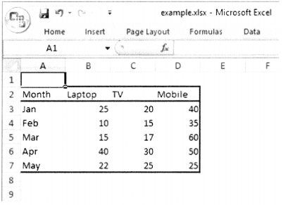
Following table 7.1 shows a ‘pricelistxsv’ represented in the form of a table. Popular word processors (MS Word, OpenOffice Writer) and spreadsheet programs (MS Excel, OpenOffice Calc) have this feature of converting text delimited by comma or any other character to a table.

No	Customer Name	Product	Price	Quantity	Total
1	Ravikumar	Laptop	25000	2	50000
2	John	TV	40000	1	40000
3	Divya	Laptop	25000	1	25000
4	Divya	Mobile	15000	3	45000
5	John	Mobile	15000	2	30000
6	Ravi Kumar	TV	40000	1	40000

As we can see, data items such as customer’s name, product’s name, and price are appearing repeatedly in the rows. This can lead to two issues: One, a manual error such as spelling or maintaining correct upper/lower case can creep up. Secondly, a change in the value of a certain data item needs to reflect at its all occurrences, failing which may lead to a discrepancy. For example, if the price of a TV goes up to 45000, the price and total columns in invoice numbers 2 and 6 should be updated. Otherwise, there will be inconsistency in the further processing of data. These problems can be overcome by using a relational database.

• Python Data Persistence – A Quick Guide
• In Python, How to Read a JSON File?
• Python Program that Reads a Text File and Counts the Number of Times a Certain Letter Appears in the Text File
• ICICIPRULI Pivot Point Calculator

SQLite installation

Installation of SQLite is simple and straightforward. It doesn’t need any elaborate installation. The entire application is a self-contained executable ‘sqlite3.exe’. The official website of SQLite, (https://sqIite.org/download.html) provides pre-compiled binaries for various operating system platforms containing the command line shell bundled with other utilities. All you have to do is download a zip archive of SQLite command-line tools, unzip to a suitable location and invoke sqlite3.exe from DOS prompt by putting the name of the database you want to open.

If already existing, the SqLite3 database engine will connect to it; otherwise, a new database will be created. If the name is omitted, an in-memory transient database will open. Let us ask SQLite to open a new mydatabase.sqlite3.

E:\SQLite>sqlite3 mydatabase.sqlite3 
SQLite version 3.25.1 2018-09-18 20:20:44 
Enter ".help" for usage hints. 
sqlite>

In the command window, a SQLite prompt appears before which any SQL query can be executed. In addition, there “dot commands” (beginning with a dot “.”) typically used to change the output format of queries or to execute certain prepackaged query statements.
An existing database can also be opened using the .open command.

E:\SQLite>sqlite3
SQLite version 3.25.1 2018-09-18 20:20:44 
Enter ".help" for usage hints.
Connected to a transient in-memory database. 
Use ".open FILENAME" to reopen on a persistent database.
sqlite> .open test.db

The first step is to create a table in the database. As mentioned above, we need to define its structure specifying the name of the column and its data type.

SQUte Data Types

ANSI SQL defines generic data types, which are implemented by various RDBMS products with a few variations on their own. Most of the SQL database engines (Oracle, MySQL, SQL Server, etc.) use static typing. SQLite, on the other hand, uses a more general dynamic type system. Each value stored in SQLite database (or manipulated by the database engine) has one of the following storage classes:

• NULL
• INTEGER
• REAL
• TEXT
• BLOB

A storage class is more general than a datatype. These storage classes are mapped to standard SQL data types. For example, INTEGER in SQLite has a type affinity with all integer types such as int, smallint, bigint, tinyint, etc. Similarly REAL in SQLite has a type affinity with float and double data type. Standard SQL data types such as varchar, char, char, etc. are equivalent to TEXT in SQLite.
SQL as a language consists of many declarative statements that perform various operations on databases and tables. These statements are popularly called queries. CREATE TABLE query defines table structure using the above data types.

CREATE TABLE

This statement is used to create a new table, specifying the following details:

• Name of the new table
• Names of columns (fields) in the desired table
• Type, width, and the default value of each column.
• Optional constraints on columns (PRIMARY KEY, NOT NULL, FOREIGN KEY)

Example

CREATE TABLE table_name ( 
column 1 datatype [width] [default] [constraint], 
column2 , 
column3..., 
 ) ;

DELETE Statement

If you need to remove one or more records from a certain table, use the DELETE statement. The general syntax of the DELETE query is as under:

Example

DELETE FROM table_name WHERE [condition];

In most circumstances, the WHERE clause should be specified unless you intend to remove all records from the table. The following statement will remove those records from the Invoices table having Quantity>5.

sqlite> select customers.name, products. name, the quantity from invoices, customers, products
...> where invoices.productID=Products.ProductID ...> and invoices.CustID=Customers.CustID;
Name               Name          Quantity
---------           ---------        ---------
Ravikumar        Laptop              2
Divya                Mobile              3
Ravikumar        Mobile              1
John                 Printer               3
Patel                 Laptop             4
Irfan                 Printer              2
Nit in Scanner 3

ALTER TABLE statement

On many occasions, you may want to make changes in a table’s structure. This can be done by the ALTER TABLE statement. It is possible to change the name of a table or a column or add a new column to the table.

The following statement adds a new column in the ‘Customers’ table:

sqlite> alter table customers add column address text (20);
sqlite> .schema customers CREATE TABLE Customers (
CustID INTEGER PRIMARY KEY AUTOINCREMENT, Name TEXT (20),
GSTIN TEXT (15), address text (20));

DROP TABLE Statement

This statement will remove the specified table from the database. If you try to drop a non-existing table, the SQLJte engine shows an error.
sqlite> drop table invoices; sqlite> drop table employees; Error: no such table: employees
When the ‘IF EXISTS’ option is used, the named table will be deleted only if exists and the statement will be ignored if it doesn’t exist.
sqlite> drop table if exists employees;

SQLiteStudio

SQLiteStudio is an open-source software from https://sqlitestudio.pl. It is portable, which means it can be directly run without having to install. It is powerful, fast, and yet very light. You can perform CRUD operations on a database using GUI as well as by writing SQL queries.

Download and unpack the zip archive of the latest version for Windows from the downloads page. Run SQLiteStudio.exe to launch the SqliteStudio. Its opening GUI appears as follows:(figure 7.3)

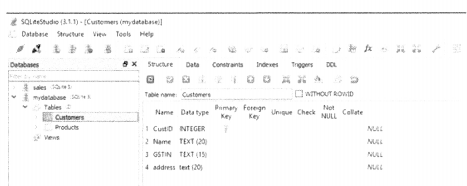
Currently attached databases appear as expandable nodes in the left column. Click any one to select and the ‘Tables’ sub-node shows tables in the selected database. On the right, there is a tabbed pane. The first active tab shows structure of the selected table and the second tab shows its data. The structure, as well as data, can be modified. Right-click on the Tables subnode on the left or use the Structure menu to add a new table. User-friendly buttons are provided in the Structure tab and data tab to insert/ modify column/row, commit, or rollback transactions.

This concludes the current chapter on RDBMS concepts with a focus on the SQLite database. As mentioned in the beginning, this is not a complete tutorial on SQLite but a quick hands-on experience of interacting with SQLite database to understand Python’s interaction with databases with DB-API that is the subject of the next chapter.