

Correlation Matrix:
Correlation matrix in python: A correlation matrix is a table that contains correlation coefficients for several variables. The correlation between two variables is represented by each cell in the table. The value ranges from -1 to 1. A correlation matrix is used to summarise data, as a diagnostic for advanced analyses, and as an input for a more complex study. The correlation’s two main components are:
Magnitude: the greater the magnitude, the stronger the correlation.
sign: If the sign is positive, this indicates that there is a regular correlation. If the value is negative, there is an inverse relationship.
In the field of Data Science and Machine Learning, we frequently encounter scenarios in which we must examine variables as well as perform feature selection. This is where Correlation Regression Analysis comes in.
correlation regression Analysis allows programmers to investigate the relationship between continuous independent variables and continuous dependent variables.
That is, the regression analysis describes the possibility and link between the data set’s independent variables as well as the independent and response (dependent) variables.
- Python Pandas Series corr() Function
- Python Program to Calculate Sum of all Maximum Occurring Elements in Matrix
- Python Program to Calculate Sum of all Minimum Frequency Elements in Matrix
The Correlation matrix is used in Correlation Regression Analysis to depict the relationship between the variables in the data set.
The correlation matrix is a matrix format that aids programmers in analyzing the relationship between data components. It denotes the correlation coefficient between a range of 0 and 1.
A positive number indicates a good correlation, a negative value indicates a low correlation, and a value equal to zero(0) indicates no dependency between the specific set of variables.
The following observations can be drawn from the Regression Analysis and Correlation Matrix:
- Recognize the relationship between the data set’s independent variables.
- Aids in the selection of important and non-redundant variables from a data source.
- Only applies to numeric/continuous variables.
Creation Of Correlation Matrix
Correlation matrix python: Here we have taken an example of a cereal dataset. Let us import and have a glance over it first.
1)Importing the Dataset
Import the dataset into a Pandas Dataframe.
# Import pandas module as pd using the import keyword
import pandas as pd
# Import dataset using read_csv() function by pasing the dataset name as
# an argument to it.
# Store it in a variable.
cereal_dataset = pd.read_csv('cereal.csv')
| name | mfr | type | calories | protein | fat | sodium | fiber | carbo | sugars | potass | vitamins | shelf | weight | cups | rating |
|---|---|---|---|---|---|---|---|---|---|---|---|---|---|---|---|
| 100% Bran | N | C | 70 | 4 | 1 | 130 | 10 | 5 | 6 | 280 | 25 | 3 | 1 | 0.33 | 68.402973 |
| 100% Natural Bran | Q | C | 120 | 3 | 5 | 15 | 2 | 8 | 8 | 135 | 0 | 3 | 1 | 1 | 33.983679 |
| All-Bran | K | C | 70 | 4 | 1 | 260 | 9 | 7 | 5 | 320 | 25 | 3 | 1 | 0.33 | 59.425505 |
| All-Bran with Extra Fiber | K | C | 50 | 4 | 0 | 140 | 14 | 8 | 0 | 330 | 25 | 3 | 1 | 0.5 | 93.704912 |
| Almond Delight | R | C | 110 | 2 | 2 | 200 | 1 | 14 | 8 | -1 | 25 | 3 | 1 | 0.75 | 34.384843 |
| Apple Cinnamon Cheerios | G | C | 110 | 2 | 2 | 180 | 1.5 | 10.5 | 10 | 70 | 25 | 1 | 1 | 0.75 | 29.509541 |
| Apple Jacks | K | C | 110 | 2 | 0 | 125 | 1 | 11 | 14 | 30 | 25 | 2 | 1 | 1 | 33.174094 |
| Basic 4 | G | C | 130 | 3 | 2 | 210 | 2 | 18 | 8 | 100 | 25 | 3 | 1.33 | 0.75 | 37.038562 |
| Bran Chex | R | C | 90 | 2 | 1 | 200 | 4 | 15 | 6 | 125 | 25 | 1 | 1 | 0.67 | 49.120253 |
| Bran Flakes | P | C | 90 | 3 | 0 | 210 | 5 | 13 | 5 | 190 | 25 | 3 | 1 | 0.67 | 53.313813 |
- protein
- fat
- sodium
- fiber
Approach:
- Import os module using the import keyword.
- Import pandas module as pd using the import keyword.
- Import numpy module as np using the import keyword.
- Import seaborn module using the import keyword.
- Import dataset using read_csv() function by passing the dataset name as an argument to it.
- Store it in a variable.
- Give the consecutive columns of the dataset as a list.
- Store it in another variable.
- Form the correlation matrix.
- Print the correlation matrix.
- Pass the above correlation matrix and annot = True as the arguments to the heatmap() function to visualize the above correlation matrix.
- The Exit of the Program.
Below is the implementation:
# Import os module using the import keyword
import os
# Import pandas module as pd using the import keyword
import pandas as pd
# Import numpy module as np using the import keyword
import numpy as np
# Import seaborn module using the import keyword
import seaborn
# Import dataset using read_csv() function by passing the dataset name as
# an argument to it.
# Store it in a variable.
cereal_dataset = pd.read_csv('cereal.csv')
# Give the consecutive columns of the dataset as a list and
# Store it in another variable.
numerc_colmns = ['protein','fat','sodium','fiber']

# Formation of the correlation matrix
corretn_matrx = cereal_dataset.loc[:,numerc_colmns].corr()
# Print the correlation matrix.
print(corretn_matrx)
# Pass the above correlation matrix and annot = True as the arguments to the heatmap() function
# to visualize the above correlation matrix
seaborn.heatmap(corretn_matrx, annot=True)
Output:
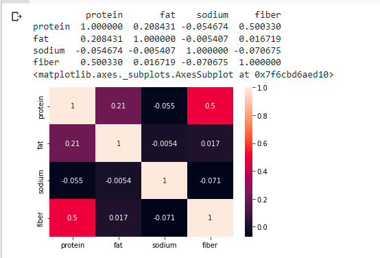
As a result of the above matrix, the following observations may be made:
With a correlation value of 1, the variables ‘protein’ and ‘fat’ are highly correlated
As a result, we can remove one of the two data variables.